An Intuitive Understanding of the Option Greeks

The Black-Scholes

I’ve decided for now to start moving my long form content to Substack, mostly to try to decomplicate life and score more eyeballs due to bothering folks in their email box.

This post originally started with the intent of explaining the monthly Gamma Exposure cycle on the indices, but I feel before we make an apple pie from scratch, we must first invent the universe. As such, before we talk about the complexities of the monthly option expiration cycle, we should probably talk first about the options Greeks.

First off, the Greeks are not real; they’re mathematical constructions that exist primarily due to the imperfection of pricing an option contract in our reality. More simply put, they arise due to rational pricing—a pretty powerful concept which allows dedicated financiers to sell you option contracts to lose money on without worrying about GME hitting $400 or some silly number like that.

What is rational pricing, exactly? In finance, rational pricing is the price of an asset assuming there is no ability to arbitrage - that is to make a risk free profit. A good example of arbitrage stems from the law of one price - that the price of an asset must hold constant around the globe. This is intuitive — if an asset X is priced at $450 in Tokyo but $800 in Des Moines, there is a risk-free way to make $350 profit (excluding import fees, transportation, etc) - you buy the asset in Tokyo and sell in Des Moines. However, assuming there is profit to be had, another individual could completely undercut you and sell the same product at $790, stealing all of your clients. You could respond and cut to $780, and so on and so on. This will continue until you reach a Nash equilibrium of zero profit (the no-arbitrage condition).

Arbitrage, or rather the lack thereof, is a critical concept in pricing assets—the understanding is that in mature, low friction markets, there should not really be ways to conduct arbitrage. Therefore, we can greatly simplify pricing assets assuming no arbitrage (this does not hold in fragmented or newer markets very well like Bitcoin, but more on that later).

The standard mechanism to price a weird, non-linear instrument like an option contract is through the argument of portfolio replication which sounds fancy but isn’t. Much like our export arbitrage example above, portfolio replication is a powerful but simple concept which states that the price of an asset, assuming no-arbitrage, should be identical to a portfolio that replicates its cash flow. That still sounds kind of big brain, so we can dumb it down a bit further. Imagine I had an asset X which gives you $10/mo for the rest of your life. How much would you pay for it? It’s a bit difficult to do discounted cash flows, so let’s imagine I had a similar asset Y which costs $200 and pays you $5/mo for the rest of your life. Now how much can X be?

Assuming equal risk here and no ability to arbitrage, the quick answer is simply $400. Why? Because $5 x 2 is $10/mo, which replicates the cash flows of Y. So an investor assuming everything else held constant should be indifferent to holding 2 of Y or 1 of X.

This nifty trick allows us to price options, even though their payouts are much more complicated than the X-Y example above:

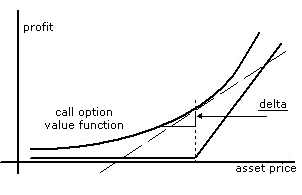
The major breakthrough of the famous Black-Scholes model was the realization that one could replicate the cash flows of an option simply by dynamically resizing a position according to the current delta of the option (which has many interpretations, one of them being the probability of the option contract ending up in-the-money). This was simply a very big deal, because it meant two things:

1) One could rationally price an option - Simply put, the minimum price of an option (per no-arb) has to be equivalent to the cost of dynamically hedging the position. If an option becomes cheaper than the cost to hedge it, the seller would simply refuse the transaction, because they would be providing liquidity at a loss.

2) It connects the options market to the equity markets - Dynamic hedging is not simply a rule of thumb to hedge an option; in the most succinct example, the hedging of the option is the option. If I were to hedge a portfolio assuming no transaction costs and frictionless buying/selling, I would expect that my ending PnL would be identical to if I had bought the option. This intuitively links the equity to the derivative, similar to understanding integration in calculus as the summation of infinitesimal rectangles (the Riemann sum).

That said, despite its popularity, Black-Scholes has many significant and profound issues. For starters, it provides a price for an option under the following conditions:

1) It assumes frictionless and costless hedging - to hedge in shares, for example, shares are discrete instruments (even accounting for fractional shares, transactions are discrete).

2) The stock pays no dividends in the lifetime of the option.

3) The stock price follows a geometric Brownian motion — or in simple terms, random walk.

4) The risk-free interest rate is constant over time.

5) Volatility is constant over time (major issue).

6) It can only really be used to suitably price European options (it assumes no early exercise is possible).

Simply put, Black-Scholes is often used as a launching ground for option pricing models in practice, but by itself is not used often. Many of its major tenets — like constant volatility — have been shown in practice to be extremely incorrect, launching the field of stochastic volatility models (where the volatility of an asset is itself modeled as a random process).

However, the important aspect of Black-Scholes is through the nifty equation we get the ability to derive the Greeks.

The Greeks look fancy, but essentially state the sensitivity of an option’s price to various factors. They’re partial differentials of the Black-Scholes equation—if you haven’t taken Calculus III, partial differentials occur because solving equations with multiple variables are hard. If you’ve taken basic Calculus, a differential is exactly what it sounds like—it’s the difference in values for some equation due to change in one variable. We can take the example of y = x + 2. When x = 5, y similarly equals 7. However, if we slide x to equal 3, y equals 5. We can fancily call this the difference, where y has changed 2 while x has also changed 2.

In Calculus, differentials are important on less well-behaved functions (like polynomials) because it allows you to reason about the instantaneous rate of change.

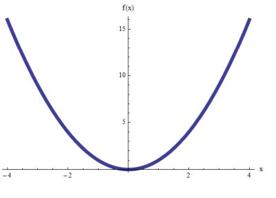
In the image above, it’s clear to see that the rate of change of y from 2 to 4 is not the same as the rate of change from 0 to 2. This is obvious with simple algebra. So similarly, the differential here cannot be a flat constant (the slope in the above example). Hence you get the idea of infinitesimal differentials, which forms the basis for derivatives in Calculus.

All the idea above here is stating is that — even though if we zoom out on the graph we can clearly see the rate of change is not constant, as we zoom in smaller and smaller we can approximate it as constant for small changes in x.

This idea analogizes to partial differentials, which is what the Greeks are to Black-Scholes. When you have multivariate equations, where every single variable can vary, you must define your infinitesimal differential based on holding other variables constant. We get some neat notation for that:

For less mathy folks, normal differentiation you get normal d, for partial differentials you get curly d.

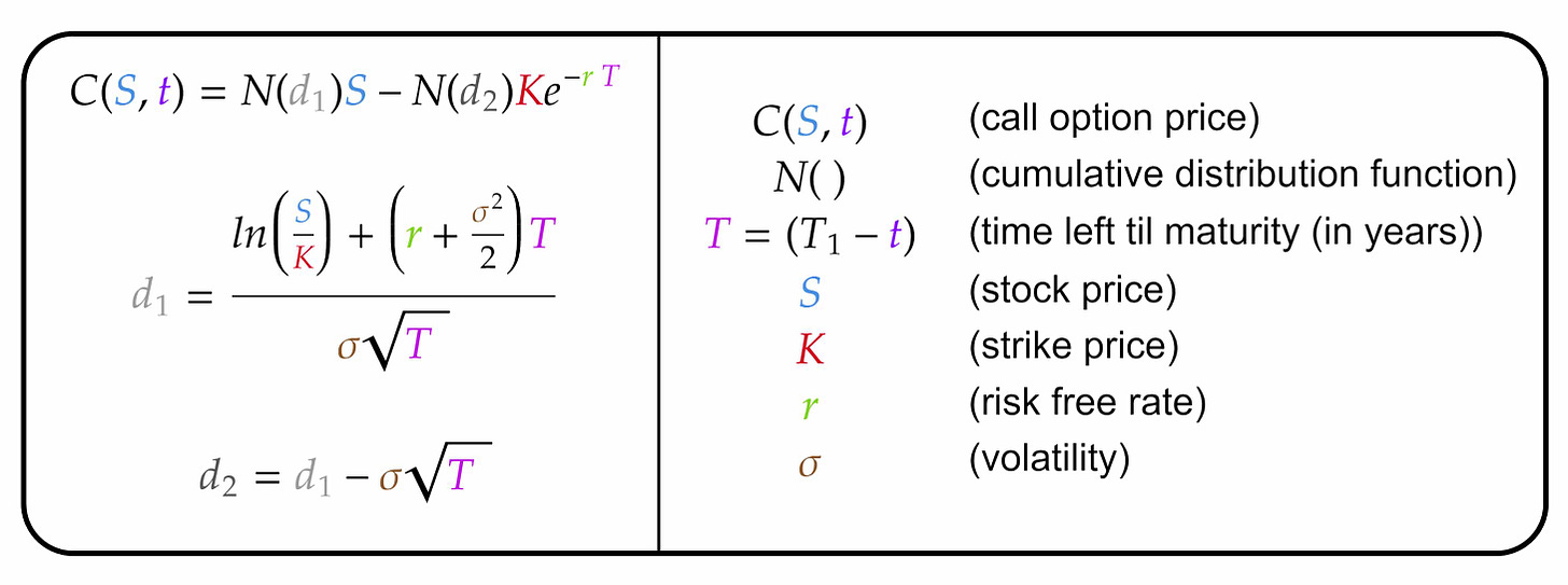
This is important because we can analyze Black-Scholes to see what variables comprise it:

Ignoring the fancy math words here like cumulative distribution function, we can see really there are four quantities which vary in our equation (the call option price is the output, and therefore isn’t varying—it’s what the other variables vary against similar to our slope example (it’s y)):

• Current stock price

• The strike price of the option contract

• The risk free interest rate

• The volatility of the asset

• The time left til maturity

So, off the bat, we know that while strike price can of course vary between contracts, by definition (at least in vanilla options) it does not vary in the lifetime of a single contract (wouldn’t it be cool if it did though). So we can immediately fix a value to that one.

For the remaining four, we get what people know as the top-level (first-order) Greeks of an options contract:

• The change of the option price as the stock price changes (we call this delta)

• The change of the option price as volatility changes (we call this vega)

• The change of the option price as the risk free interest rate changes (we call this rho)

• The change of the option price as the time left to maturity changes (we call this theta).

From looking at the equation and a pretty rudimentary understanding of calculus, we can simply derive all the first-order Greeks. Pretty sweet, right?

In the next post, I’m going to delve into more the meaning of the first and second order Greeks, and finally in the third post I’ll talk about the more advanced concepts relating it to the behavior of the market and the monthly OPEX cycle.

As I mentioned in my weekly forecast, I’m going to start moving to a paid model for long-form content, where I release it as part of the subscription service on Substack. This is to raise money for charity—although as I explained, I will take a fraction to cover potential taxes arising from it (I will post the totals publicly as well as charity receipts as well).

At least for the foreseeable future, my weekly forecast will remain free, since I enjoy doing it. If you’d like to subscribe at any time, check it out here.

https://nopeitslily.substack.com/subscribe

And feel free to also give me charity recommendations! I’ll change it up from time to time according to where I think it could be best distributed, and will have to valid it is using money effectively (e.g. Charity Navigator). It also will of course have to be a registered charity (for taxation purposes).

Cheers,

Lily